
B+ Trees#
The problem with BSTs#
\(\log(n)\) is fast, so we are quite pleased with our BSTs for our add and
contains functions (and their Map equivalents). However, we have been making
a couple assumptions. We’ve assumed that every piece of data is equally quick
to read, and that our data fits in memory (RAM). When we get into
database-sized data though, we start having to put data on the disk (like an
SSD or HDD). Reading from disk is far, far, far slower than reading from RAM,
and even only a dozen disk accesses will be noticeable in database
performance. So, while this is “only a coefficient,” it’s a coefficient we’re
forced to reckon with in certain cases.
In a database, data is read from the disk in chunks called pages or blocks. A single disk read fetches one entire block into memory. A BST node is small, typically holding one key and pointers to two children, which is far smaller than a block. When stored on disk, these nodes can be scattered all over. Traversing the tree from the root to a leaf might require reading a different disk block for every single node in the path. If a BST is 15 levels deep, a single search could require 15 separate disk reads in the worst case. Given that a disk read is a huge performance bottleneck, this is unacceptable for a database that needs to perform thousands of operations per second. Even for a balanced BST with \(N\) items, a search takes \(O(\log N)\) node visits, which translates to a costly \(O(\log N)\) disk reads.
BSTs are also not optimized for range queries. As you know, databases frequently handle range queries like “find all employees with a salary between $50,000 and $70,000.”
BST Traversal: To perform a range query on a BST, you have to perform an in-order traversal between the start and end points of the range. This involves traversing up and down the tree, jumping between parent and child nodes, which again can lead to numerous, scattered disk reads. The nodes containing the data you want are not stored sequentially.
The B+ Tree#
B+ Trees are designed to address these shortcomings and allow very fast range queries with very large amounts of data (where “very fast” means both “few operations” and “few disk accesses”). Here’s a picture of a B+ tree for reference.
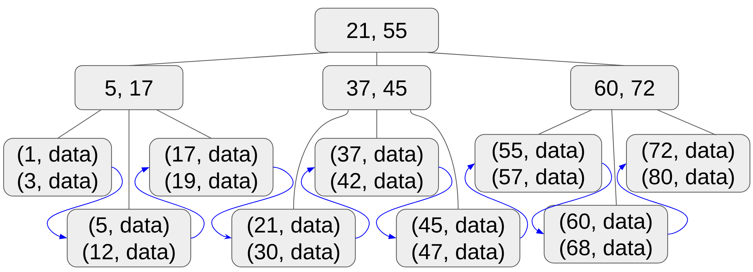
The first thing to note is the leaves. As you reference the image, note that for space reasons, the leaves are the bottom two rows of nodes shuffled together.
Every key-value pair appears in a leaf. None appear in interior nodes.
Every leaf contains multiple key-value pairs. In fact, the goal is for a leaf to be close to a page in size, so a leaf normally contains hundreds or thousands of key-value pairs (but I can’t draw that, so I only put two per leaf). This is this way so that one disk access pulls up as much data as possible.
The key-value pairs are arranged in sorted order.
Leaves are linked together as a linked list (blue arrows), so that you can find the next key-value pair without re-navigating the tree.
The interior nodes consist only of keys. I’ve drawn this tree where each node contains 2 keys, and the tree has a branching factor of 3. The leftmost child contains data less than the smallest key, the middle child contains data greater than or equal to the smaller key and smaller than the bigger key, and the right child contains data greater than or equal to the bigger key. Like the leaves, in reality, each interior node would contain about a page of data, meaning the branching factor would be in the hundreds or thousands. When searching for a key-value pairs, we can figure out which child it is in by performing binary search on the array of keys.
Executing range()#
So, to execute a range(small, big) query, we set out to search for the
small key. We start with the root, and perform binary search to identify
which child would have the small key. We navigate to that child. If it’s not
a leaf, we again perform binary search to identify which child would have that
key. Once we reach the leaf, we do binary search to find the small key-value
pair, and then navigate rightward along the linked list of leaves until we
find the big key, and return a list of all the key-value pairs between the
two.
The search for small is still logarithmic, but because we are replacing much
of the node navigation with binary search on large arrays, we are minimizing
disk accesses.
Building a B+ tree#
To insert an element into a B+ tree, we navigate to the relevant leaf. If the leaf has room for another key-value pair without outgrowing a page, load it into RAM, add the element to the sorted array, and then put the leaf back into disk.
If a leaf is full, we split it into two leaves, and promote the smallest key of the new right node to the interior node above it.
If the interior node is full, we split it also into two nodes, and promote the smallest key of the new right node to the level above it.
You can follow along with these processes with this great visualization from USF.