Binary Search Trees

Trees are often used to implement Sets and Maps, using Binary Search Trees (BSTs). A BST is a Binary Tree, meaning that each node has up to two children:

class SetNode:
  def __init__(self, data):
    self.data = data #were this a MapNode, it would have a self.key and
                     # self.value, or a self.keyvalue, which would be a
                     # tuple of key and value
    self.left = left
    self.right = right

Adding to a BST

For simplicity’s sake, we’ll assume you’re implementing a Set. Here I demonstrate how a BST can be constructed as the user makes several calls to add(e) to an initially empty BST.

bst.add(7)

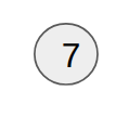
7 is added as the root node of the tree.

bst.add(9)

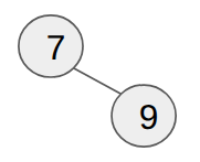
9 is larger than 7, so it goes to the right of the root and becomes its right child.

bst.add(4)

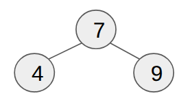
4 is smaller than 7, so it goes to the left of the root and becomes its left child.

bst.add(6)

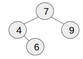
6 is smaller than 7, so it goes to the left of the root. 6 is larger than 4, so it goes to the right of the node containing 4, and becomes its right child.

bst.add(2)

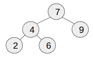
2 is smaller than 7, and smaller than 4, so it becomes 4’s left child.

bst.add(3)

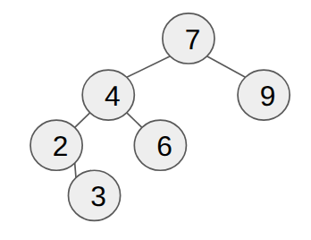
3 is smaller than 7, smaller than 4, and larger than 2.

We can implement this recursively:

class BST:
  def __init__(self):
    self.root = None

  def _add(self, node, e):
    if node is None:
      return SetNode(e)
    if e==node.data:
      return node
    elif e < node.data:
      node.left = self._add(node.left, e)
    else:
      node.right = self._add(node.right, e)
    return node

  def add(self, e):
    self.root = self._add(self.root, e)

Searching for data in a BST

For .contains(e) or .get(k), we have to find a node in a binary search tree. This is very easy - if the thing you’re looking for is smaller than the current Node’s data, it must be in its left subtree. If it’s larger, it’s in the right subtree.

def _contains(self, node, e):
  if node is None:
    return False # We made it to the end of the tree without finding it
  elif node.data == e:
    return True # We found it!
  elif e < node.data:
    return self._contains(node.left, e)
  else
    return self._contains(node.right, e)

def contains(self, e):
  return self._contains(self.root, e)

Traversal

For our linked lists, we had a “recipe” for traversal, which means visiting each node. It looked like this:

def _ll_traverse(self, node):
  if node is None:
    return
  # Location A
  self._ll_traverse(node.next)
  # Location B

Recall that any code that exists in Location A will occur from the front to the back of the linked list. Any code that exists in Location B will occur from the back to the front.

We’ll frequently want to traverse trees, as well. Our Binary Tree traversal looks like this (and is definitely something we want to do recursively):

def _tree_traverse(self, node):
  if node is None:
    return
  # Location A
  self._tree_traverse(node.left)
  # Location B
  self._tree_traverse(node.right)
  # Location C

Now we have three places to do work, and it is useful to get good at thinking about what the results of them would be. Suppose we put print(node.data) in Location A. This is called preorder traversal. Location B is inorder traversal, and Location C is postorder traversal.

Consider this tree again:

The three different traversals, run on this tree, would result in operating on these nodes in the following order:

• Preorder: 7,4,2,3,6,9

• Inorder: 2,3,4,6,7,9

• Postorder: 3,2,6,4,9,7

It is important you be able to run through these traversals on any given tree.

Runtimes of Set and Map operations with a BST

In all the Set and Map operations, in the worst case, the relevant nodes are at the bottom of the tree, so the runtimes are equivalent to the height of the tree. So, how tall are trees?

It is possible to arrange tree data so that it is a glorified linked list. For example, suppose we construct a BST by adding numbers in increasing order - the tree will consist of only right children, making it \(O(n)\) in height. Data in this order is not very uncommon.

Fortunately, we have lots of variations of BSTs we can use to overcome this potential weakness, such as AVL Trees and Red-Black Trees. For this major, it is not actually important that we understand the details of how these trees work - the important thing is that we understand that it is possible to perform additions and removals in such a way that we can guarantee that the tree will remain \(O(\log(n))\) in height.

So, all Set and Map operations are \(O(\log(n))\).